CPS3 (case and workaround)

There is a case that user open cps3 modul then open formula under grid operation. CPS3 will be always kicked out or hang.

Please try:

• Go to the Project Directory , rename user’s session file “<user_name>.1cps” to <user_name>.1cps_copy (under directory project /CPS3)
• Go to user’s home directory, under the home directory go to subdirectory . Type “cd  .cps” (it’s hidden directory) and seek file of formula *.frm
• Rename all formula file to a new name, e.g.  mv formula.frm formula.frm_original
• Start CPS3 normally

Gross Rock Volume (GRV)

Gross Rock Volume (GRV)

Gross rock volume (GRV) is total volume of reservoir that bounded by top of the reservoir, base reservoir and oil water contact (OWC)/gas water contact (GOC). The contact is called also as structural spill point (SSP) which determine how level of the hydrocarbon content can fill in the reservoir before spilling out to other place die to structural control.
GRV calculation is used in volumetric evaluation of the hydrocarbon content in the reservoir.

To be continued…

Seismic Attribute

Seismic attribute simply can be defined as any information derived from seismic data. It’s just seismic data it’s self but viewed from different point of view both by direct measurement, computing, etc.

Seismic attribute is used as some seismic anomaly can not be identified clearly with the usual seismic data. So by using seismic attribute, the anomaly will be more clear and easily detected so that interpretation become more true and fit with the real condition.
Mathematically, seismic signal can be written as a formula:

u(t) = x(t) + i (y(t)

where:

x(t) is seismic data conventional which usually used for seismic interpretation
y(t) is a quadrature derived by shifting x(t) by 90 degree
u(t) can be obtained by doing Hilbert Transform to seismic data where real component is the seismic data it’s self and imaginer component is the quadrature.

Some kind of seismic attribute is instantaneous energy (envelope), instantaneous phase, instantaneous frequency, etc

How to load log curves into GF project

By Arif U hakim

Step by step workflow to load log curves in las format:

1. Select GF project

2. Select application or data management (well project only)

3. Click Loaders and Unloaders

4. Click ASCII Load

5. Input files

6. If it’s LAS file, select in control file format “las depth”

7. Select traget field, target well and borehole

8. run

Notes: there is special trick to load selected log curves in las files as follows:

– Create control file (not using las depth format)

– Set the start row and stop raw from the data

– set the number of column

– use explicit and type MD

– Add arrays with the log curves name that will be loaded (for example VCL, PIGN and SUWI). Fill in the righ column based on las data and the correct unit

– Click OK and run

 

 

Mount Media into Linux

If we connect the removeable media (external usb, etc) to linux machine, it wont be detected directly until we mount it using unix/linux commands. Here are the step by step:

(login as root)

>> su –

Seek for a disk to attach/mount

>> cd /disk or cd /tmp

>> fdisk -l  –> result in /dev/sdcl

>> mount  -t  ntfs-3g  /dev/sdcl  /disk

To unmount

>> cd /

>> umount /disk

 

How to load fault in OpenWorks

Case:

You have data with format like this:

AR02059               6938.       380.     1      1     1        #UAS#                             2
AR02059               6933.       907.     1      1     2        #UAS#                             2
AR02059               6938.       1734.   1      1     2        #UAS#                             2
AR02059               6976.      2521.    1      1     3        #UAS#                             2
AR02059               6854.      377.      1      1      1       #UAS#                             2
AR02059               6849.      889.       1      1      2       #UAS#                             2

How to load it?

Step:

1. Create format like this (its also provided in /l/sys/ow200312/sw_project/ —> named: trsp.fault_fmt).

FAULT_NAME 1 50
FAULT_PTYPE 52 52
FAULT_LINEID 54 63
FAULT_TRACE 65 74
FAULT_SHOTPOINT 76 85
FAULT_Z 87 96
FAULT_COLOR 98 100
FAULT_TYPE 102 104

Save it!

2. Draw a fault then export with above format in every line in seismic section to get the FAULT_LINEID

The result will be:

jkr_test                                           1    166.000              7321.011       716.000         4                       1
jkr_test                                           3    166.000              7415.000      1324.000      4                        1

(fault name)             (fault ptype) (fault_lineID)     (fault SP)       (fault_Z)   (fault color)   (fault_type)

FAULT_TRACE –> not written/output here

3. Take the FAULT_LINEID to edit the data above and give name of the fault example: ArafuraSeaIIFault

AR02059     6938.0      380.0     1        2 ArafuraSeaIIFault
AR02059     6933.0      907.0     2        2 ArafuraSeaIIFault
AR02059     6938.0     1734.0     2       2 ArafuraSeaIIFault
AR02059     6976.0     2521.0     3       2 ArafuraSeaIIFault
AR02059     6854.0      377.0     1        2 ArafuraSeaIIFault
AR02059     6849.0      889.0     2        2 ArafuraSeaIIFault
Change the first column (LINE NAME) becomes FAULT_LINEID from step 2 because OW can not load using LINE NAME but load FAULT_LINEID

The final result must be like this:

205     6938.0      380.0     1        2 ArafuraSeaIIFault
205     6933.0      907.0     2        2 ArafuraSeaIIFault
205     6938.0     1734.0     2       2 ArafuraSeaIIFault
205     6976.0     2521.0     3       2 ArafuraSeaIIFault
205     6854.0      377.0     1        2 ArafuraSeaIIFault
205     6849.0      889.0     2        2 ArafuraSeaIIFault
“205” is FAULT LINEID

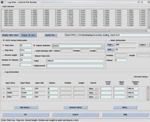
4. Create new format for loading is as follows:

FAULT_LINEID 1 12
FAULT_SHOTPOINT 15 23
FAULT_Z 26 34
FAULT_PTYPE 39 40
FAULT_TYPE 48 49
FAULT_NAME 50 67

1-12, 15-23 can be set based on the ascii data.

Save it to example:

hakimau_fault_ugm.fault_fmt (extension is fault_fmt).

5. You are DONE!!!!!!

====================================

If you do Export Import with Default or TRSPH format, PAY ATTENTION TO NO OF COLUMN. If you change the column position, it wouldnt work coz the column number shift and not match again with the original format.

Convert Velocity from Handvel to XYTV format

By Arif U Hakim

If you have Handvel format like this:

HANDVEL   11002869 1470947.2 9338609.0        12      2880
64      1572    258     1550    408     1650    663     1850
836     2127    1176    2589    1960    3610    2592    4050
3920    4570    7581    5450    9944    5790
HANDVEL   11002949 1470027.2 9338189.0        12      2960
60      1581    283     1567    408     1650    684     1875
874     2161    1152    2577    1392    2874    1608    3150
1948    3615    2960    4250    3904    4630    7396    5670
9888    6209

You can use this script to convert:

Type it in “nedit”, save it (example “arif.sh”) and run by typing —–> ./arif.sh vel_name.dat > vel_name_converted.dat

************************************************************

#!/bin/sh

awk ‘
/HANDVEL/ {
funcid = $2
x = $3
y = $4
}
$0 !~ /HANDVEL/ {
for (i = 2; i <= NF; i=i+2) {
printf “%10s %10s %10s %10s %10s\n”, funcid, x, y, $(i-1), $i
}
}
‘ $1

**************************************************************

The result will be:

11002869  1470947.2  9338609.0         64       1572
11002869  1470947.2  9338609.0        258       1550
11002869  1470947.2  9338609.0        408       1650
11002869  1470947.2  9338609.0        663       1850
11002869  1470947.2  9338609.0        836       2127
11002869  1470947.2  9338609.0       1176       2589
11002869  1470947.2  9338609.0       1960       3610
11002869  1470947.2  9338609.0       2592       4050
11002869  1470947.2  9338609.0       3920       4570
11002869  1470947.2  9338609.0       7581       5450
11002869  1470947.2  9338609.0       9944       5790
11002949  1470027.2  9338189.0         60       1581
11002949  1470027.2  9338189.0        283       1567
11002949  1470027.2  9338189.0        408       1650
11002949  1470027.2  9338189.0        684       1875
11002949  1470027.2  9338189.0        874       2161
11002949  1470027.2  9338189.0       1152       2577
11002949  1470027.2  9338189.0       1392       2874
11002949  1470027.2  9338189.0       1608       3150
11002949  1470027.2  9338189.0       1948       3615
11002949  1470027.2  9338189.0       2960       4250
11002949  1470027.2  9338189.0       3904       4630
11002949  1470027.2  9338189.0       7396       5670
11002949  1470027.2  9338189.0       9888       6209

 

Miscellaneous in CKS/VSP Report

By Arif U Hakim

A. Example 1 of Checkshot report Table in VSP report :

[ CHECKSHOT REPORT] by Sclumberger

1. Level Number

2. Vertical Depth from SRD

3. Measured Depth from KB

Transfer colormap between IESX

One of the usage of colormap (colorbar) in IESX is while displaying seismic in a seismic section. It can be time consuming if users set up new colormap while the seismic will be displayed is the same class but in other project.

To transfer colormap between iesx, here is the workflow:

1. Select Project

2. Click Application Manager -> Data

3. Click Colormap

4. Select the colormap and click Arrow Down

5. Give a exported name in directory destination

To import is just click Arrow Up and select the colormap file then click OK

export-import-colormap

Some Kinds of Velocity

by Arif U Hakim

There are at least 5 kinds of velocity commonly used by interpreter to build velocity modeling or time-to-depth conversion.

1. Stacking Velocity

The distance-time relationship determined from analysis of normal moveout (NMO) measurements from common depth point gathers of seismic data. The stacking velocity is used to correct the arrival times of events in the traces for their varying offsets prior to summing, or stacking, the traces to improve the signal-to-noise ratio of the data.

2. RMS Velocity